Distributed Search in Synchronous Networks
A BFS tree basically optimizes the communication time from a process at a distinguished node to all other processes in the network.
(BFS, Bellman-Ford in Distributed Network, read and summarized from the book Distributed Algorithms by Nancy A. Lynch)
Synchronous Network
Breadth-First Search
n: Total number of nodes in the network
diam: Diameter of the network
E: number of (directed) edges in the network
A BFS tree helps optimize the communication time from a process at a distinguished node to all other processes in the network.
The BFS problem and its solution somehow become simpler when all connections between pairs of nodes in the network are bidirectional, meaning the network graph is undirected.
Problem
We define a directed spanning tree of a directed graph G = (V,E) as a rooted tree that consists of edges of E, with all edges directed from parent to child, and that includes every vertex of G. A directed spanning tree of G with root node i is a breadth-first one if each node at distance d from i in G appears at depth d in the tree (that is, at distance d from i in the tree).
For the BFS problem, we assume the network connections between nodes are stable and there is a source node i0. We need an algorithm that outputs a breadth-first directed spanning tree of the network graph, rooted at i0.
As usual, processes only communicate with each other over edges. Processes are assumed to have their own UID, but they don’t know the size of the network or other parameters about its extent.
SynchBFS
The basic idea of the algorithm we need is quite similar to the traditional BFS algorithm. We call this algorithm SynchBFS.
The SynchBFS algorithm: At any point in time, there is a set of “marked” processes, starting with process i0. Process i0 sends a search message in round 1 to all the nodes around it. In any round, if an unmarked process receives a search message, it marks itself and picks the process that sent that search message as its parent. After each process is marked, it also continues to send search message to all the nodes around it.
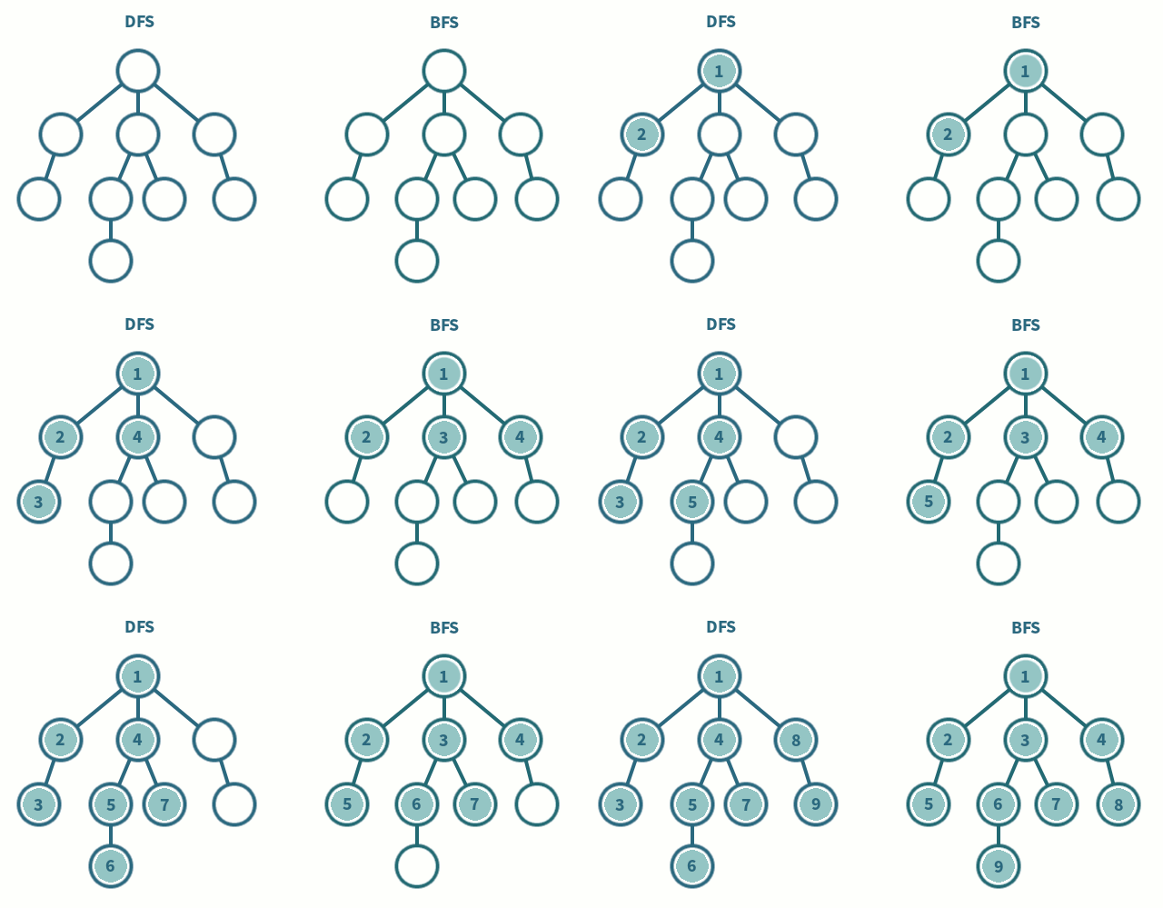
It’s not hard to see that SynchBFS produces a BFS tree. To argue this, we can state an invariant: after r rounds, every process at distance d from i0 in the network graph, 1 <= d <= r, has its parent already defined. As usual, this invariant is tied to the number of rounds.
-
Complexity analysis: The time complexity is O(diam), it takes diam rounds. The number of messages sent is |E|.
-
Reducing the communication complexity: As with the FloodMax algorithm, reducing the number of messages is possible (I haven’t read FloodMax yet so I don’t understand this part)
-
Message broadcast: SynchBFS can be used to broadcast messages in the network (since the SynchBFS tree already covers all nodes in the network), in which case the node that wants to broadcast is the root.
-
Child pointer: WIP
-
Termination: Sending a “done” message from the leaf nodes up to the root can be done by sending from children to parents one level at a time. This process is called
convergecast.
Applications
Breadth-first Search is one of the building blocks for distributed algorithms. Below are some applications where SynchBFS can be used or extended to carry out other operations in a distributed system.
Broadcast: As mentioned above, one of the most common uses of BFS in a distributed system is to reduce the resources spent on broadcasting between nodes. Once the BFS tree has been built (mapped onto the nodes in the network), the time needed to broadcast a message is O(diam).
Global computation: Another use of the BFS tree in a distributed system is computing over the results from every node. For example: each process has a positive integer, and we need to find the sum of all these numbers across the network. With a BFS tree, this is solved simply and efficiently as follows. Each child node sends its value to its parent, the parent waits until its children have sent all their integers, adds them up, and sends the result to its own parent. The needed value quickly reaches the root node of the BFS tree.
Electing a leader: Using SynchBFS, an algorithm can be designed to elect a leader node in a network with UIDs, even when the processes know nothing about n or diam. Specifically, all processes in the network can initiate breadth-first search trees in parallel at the same time. Similar to Global computation, the root node is elected as the leader. If the graph is undirected, the time needed is O(diam) and the number of messages is O(diam * |E|).
Shortest Path
As mentioned above, we use the BFS tree to describe the nodes in the network, with the goal of creating a structure that makes communication between nodes (broadcast communication) convenient. __ When sending messages, we always want the shortest path with the lowest communication cost between 2 nodes => Finding the shortest path, which reduces to the shortest path problem in a graph. This is a very familiar problem for anyone who has studied Graphs. To solve it, there are many algorithms and variants so far, the most popular being Dijkstra and Bellman-Ford.
 (illustration: Dijkstra on top and Bellman-Ford below)
The Bellman-Ford algorithm applied in a distributed network:
(Distributed Bellman-Ford in a message passing way 😏)
Each node gets the optimal routing table by exchanging routing tables with other nodes. When exchanging, a node sends a message to other nodes, and the message contains:
- Origin: The value (UID) of the node sending this message
- Routing Table: The Routing Table the sending node currently has
class Node(object):
    def __init__(self, name):
        self.name = name
        self.routing_table = {}
        self.routing_table[self.name] = 0

    # the message contains
    # - origin
    # - routing_table
    def process_message(message):
        # Get the cost from the receiving node to the node that sent the message
        cost = self.get_cost(self.name, message['origin'])
        # Iterate over all nodes in the routing table of the sending node
        # u: is a node, c is the cost to reach that node in the routing table
        for u, c in message['origin'].routing_table.items():
            if u in self.routing_table:
                # Update the routing table following the Bellman-Ford algorithm
                # If the current cost to that node is greater than the sum of the cost to the sending node and the cost in the routing table, the receiving node's routing table is updated
                if cost + c < self.routing_table[u]:
                    self.routing_table[u] = cost + c
            else:
                # If this node doesn't know node u, it is added to the receiving node's routing table
                self.routing_table[u] = cost + c
The algorithm is pretty simple. When a node receives a message, it iterates over all the nodes in the sending node’s routing table. If the current cost to that node is greater than the sum of the cost to the sending node and the cost in the routing table, the receiving node’s routing table is updated.
At the start, each node’s routing table has the values shown in the figure below:
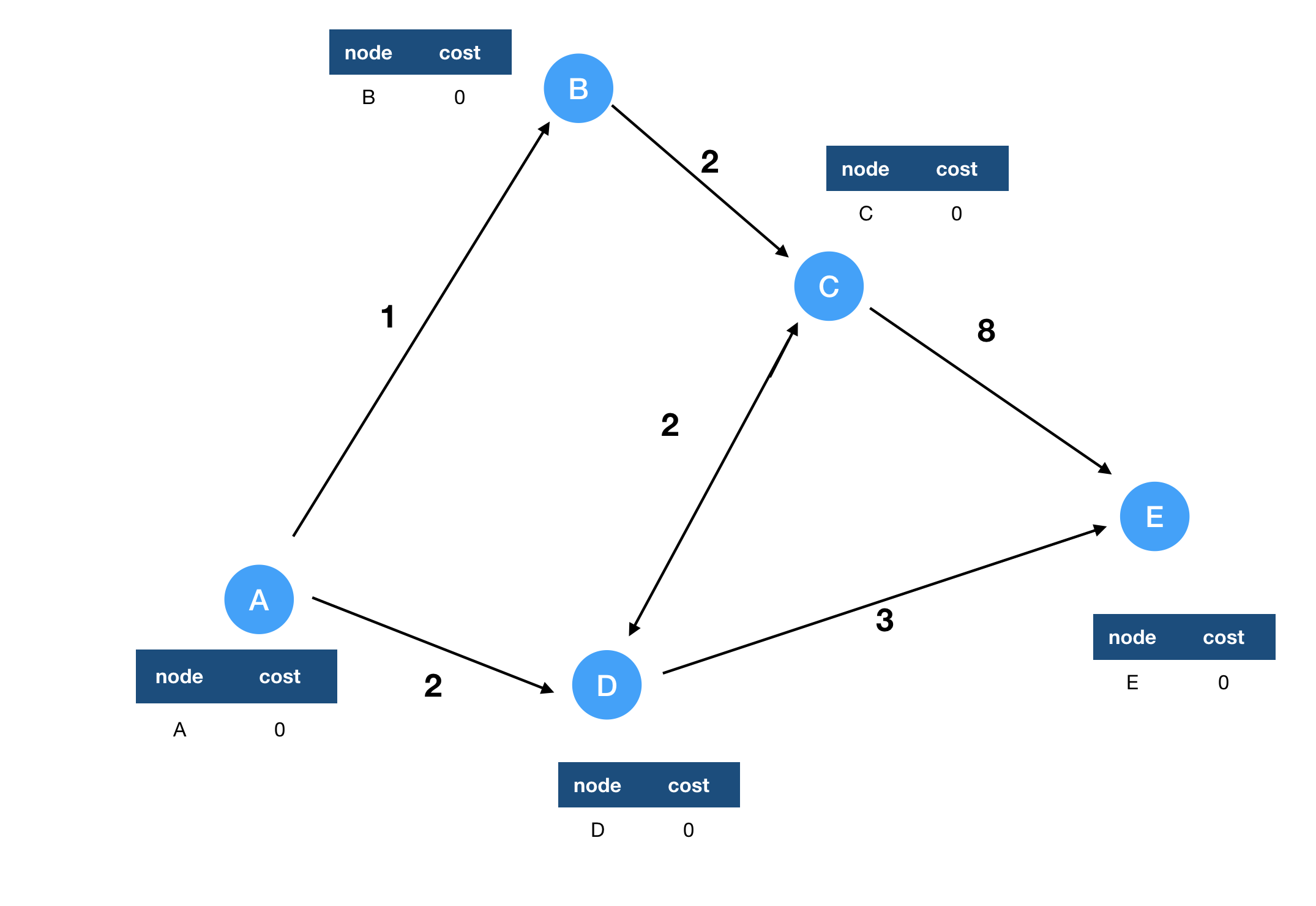
In the next step, node A receives messages from nodes B and D along with their routing tables. After receiving those 2 messages, A updates its routing table as follows:

The other nodes similarly process the messages sent from their neighbors. After that, the routing tables on the nodes look like this:
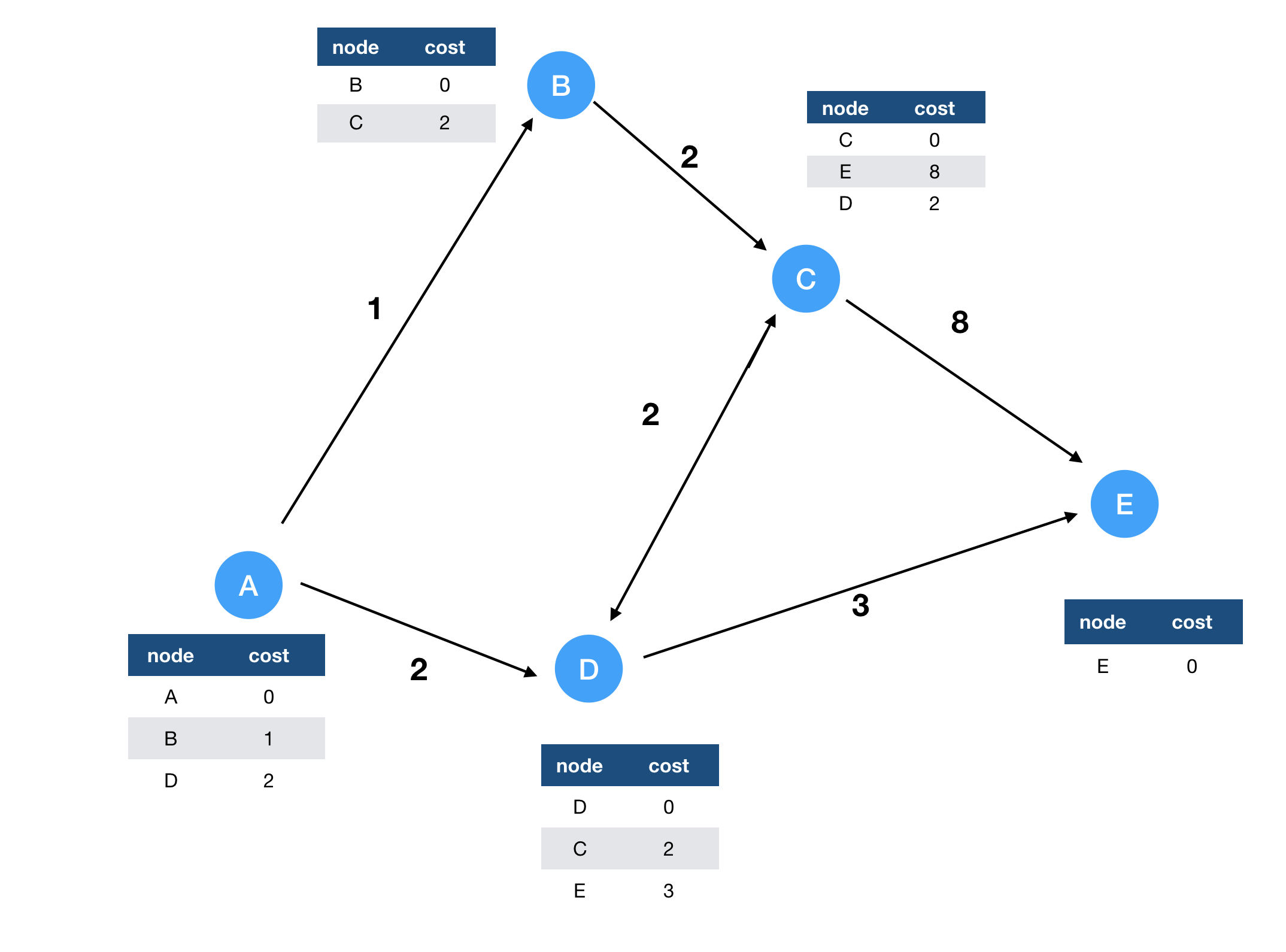
Because C doesn’t receive a message from any node, its routing table isn’t updated. The other connected nodes still receive routing tables from their neighbors and keep updating theirs.
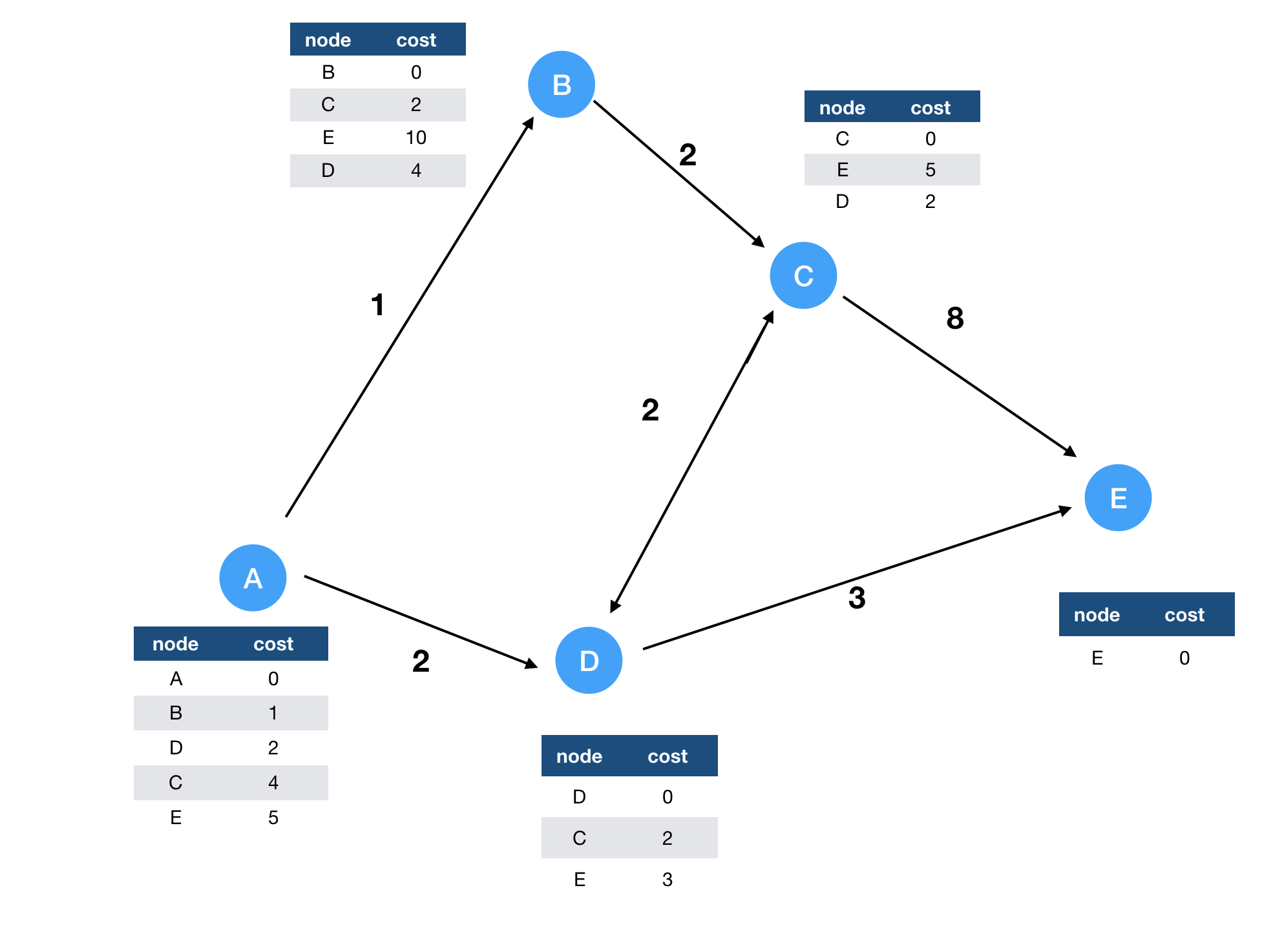
Since C receives a message from D about routing to E, C knows it can reach E through D with a cost of 5. B then also updates its (non-optimal) routing table based on C. After each round, the routing tables get updated and the shortest distances in them converge toward the optimal values.
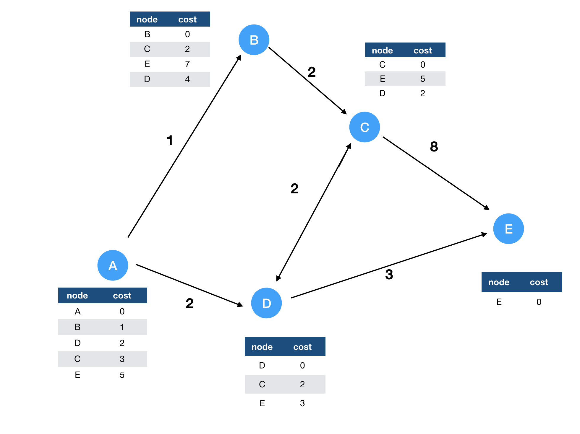
As we can see, after n - 1 rounds the values in the routing tables are optimal.
*Note: A cycle with negative total cost can cause infinite iteration (each pass around the cycle reduces the path length, and the more you traverse the lower it gets, so it goes on forever).
Complexity: The time complexity of the Bellman-Ford algorithm is n - 1, and the number of messages is (n - 1) * |E|.
Asynchronous Network
WIP